A practical problem with eigenvector centrality is that it works well only if the graph is (strongly) connected. Real undirected networks typically have a large connected component, of size proportional to the network size. However, real directed networks do not. If a directed network is not strongly connected, only vertices that are in strongly connected components or in the out-component of such components can have non-zero eigenvector centrality. The other vertices, such as those in the in-components of strongly connected components, all have, with little justification, null centrality. This happens because nodes with no incoming edges have, by definition, a null eigenvector centrality score, and so have nodes that are pointed to by only nodes with a null centrality score.
A way to work around this problem is to give each node a small amount of centrality for free, regardless of the position of the vertex in the network. Hence, each node has a minimum, positive amount of centrality that it can transfer to other nodes by referring to them. In particular, the centrality of nodes that are never referred to is exactly this minimum positive amount, while linked nodes have higher centrality. It follows that highly linked nodes have high centrality, regardless of the centrality of the linkers. However, nodes that receive few links may still have high centrality if the linkers have large centrality. This method has been proposed by Leo Katz (A new status index derived from sociometric analysis. Psychometrika, 1953) and later refined by Charles H. Hubbell (An input-output approach to clique identification. Sociometry, 1965). The Katz centrality thesis is then:
A node is important if it is linked from other important nodes or if it is highly linked.
Let $A = (a_{i,j})$ be the adjacency matrix of a directed graph. The Katz centrality $x_{i}$ of node $i$ is given by: $$x_i = \alpha \sum_k a_{k,i} \, x_k + \beta$$ where $\alpha$ and $\beta$ are constants. In matrix form we have: $$x = \alpha x A + \beta$$ where $\beta$ is now a vector whose elements are all equal a given positive constant. Notice that the centrality vector $x$ is defined by two components: an endogenous component that takes into consideration the network topology and an exogenous component that is independent of the network structure. It follows that $x$ can be computed as: $$x = \beta (I - \alpha A)^{-1} = \beta \sum_{i=0}^{\infty} (\alpha A)^i $$ Form the last equivalence it is clear that the Katz status of a node is defined as the number of weighted paths reaching the node in the network plus an exogenous factor, a generalization of the in-degree measure which counts only paths of length one. Notice that long paths are weighted less than short ones by exploiting the attenuation factor $\alpha$. This is reasonable since endorsements devalue over long chains of links.
The free parameter $\alpha$, known as the damping factor, should be chosen with case. For small (close to 0) values of $\alpha$ the contribution given by paths longer than one rapidly declines, and thus Katz scores are mainly influenced by short paths (mostly in-degrees) and by the exogenous factor of the system. When the damping factor is large, long paths are devalued smoothly, and Katz scores are more influenced the by endogenous topological part of the system. It is recommended to choose $\alpha$ between $0$ and $1 / \rho(A)$, where $\rho(A)$ is the largest eigenvalue of $A$ (the measure diverges at $\alpha = 1/ \rho(A)$).
Interestingly, it is possible to assign to each node $i$ a different minimum amount of status $\beta_i$. Nodes with higher exogenous status are, for some reason, privileged from the start. For instance, in the setting of the Web, we might bias the result towards topics, like contemporary art or ballet, that are of particular interest to the user to which the Web page ranking is served.
If the network il large, inverting matrix $I - \alpha A$ might be prohibitive, hence a direct method for the computation of centralities is preferable: Let $x^{(0)}$ be an arbitrary vector. For $k \geq 1$, repeatedly compute $x^{(k)} = \alpha x^{(k-1)} A + \beta$ until convergence. Notice that if $A$ is sparse, then $I - \alpha A$ is sparse, and hence each vector-matrix product can be performed in linear time in the size of the graph.
The built-in function alpha.centrality (R) computes Katz centrality.
A user-defined function katz.centrality using the solve R function follows:
# Katz centrality
# INPUT
# g = graph
# alpha = damping factor
# beta = exogenous vector

katz.centrality = function(g, alpha, beta) {
  n = vcount(g);
  A = get.adjacency(g);
  I = diag(1, n);
  c = beta %*% solve(I - alpha * A)
  return(as.vector(c))
}
An alternative user-defined function katz.centrality using a direct computation is the following:
# Katz centrality (direct method)
# INPUT
# g = graph
# alpha = damping factor
# beta = exogenous vector
# t = precision
# OUTPUT
# A list with:
# vector = centrality vector
# iter = number of iterations

katz.centrality = function(g, alpha, beta, t) {
  n = vcount(g);
  A = get.adjacency(g);
  x0 = rep(0, n);
  x1 = rep(1/n, n);
  eps = 1/10^t;
  iter = 0;
  while (sum(abs(x0 - x1)) > eps) {
    x0 = x1;
    x1 = as.vector(alpha * x1 %*% A) + beta;
    iter = iter + 1;
  }
  return(list(vector = x1, iter = iter))
}
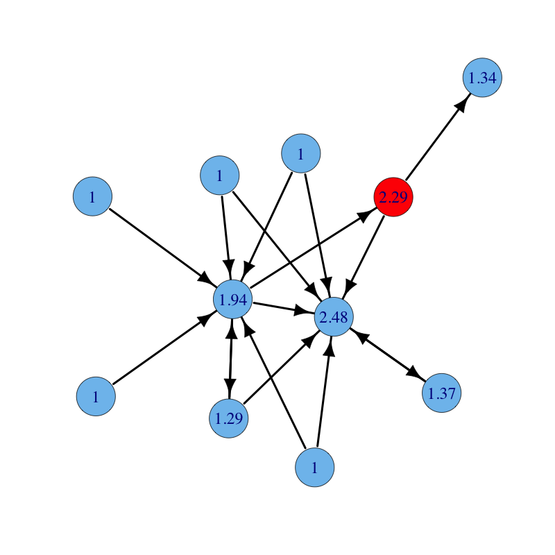
A directed graph with nodes labelled with their Katz centrality ($\rho(A) = 1$). Parameters are: $\alpha = 0.85$ and $\beta = 1$:
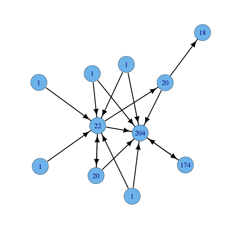
The same graph with parameters $\alpha = 0.15$ and $\beta = 1$ (long paths give less contribution):
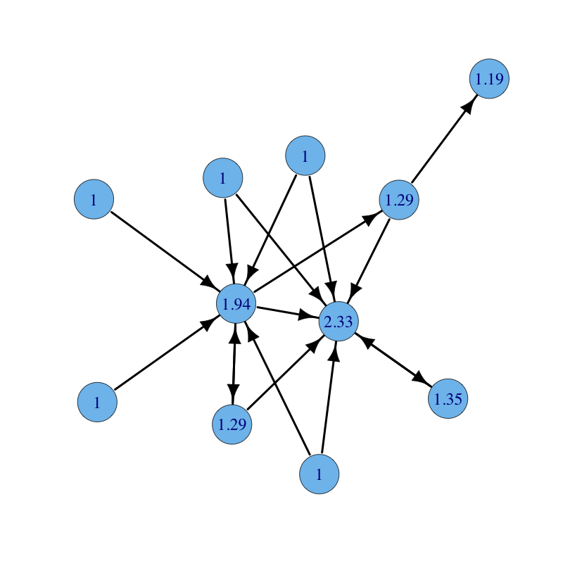
The same graph with parameters $\alpha = 0.15$ and $\beta = 1$ for all nodes but the red node for which $\beta = 2$ (notice how the red node and all nodes reachable from it increase their centrality):